CEACT (Cost-Effectiveness Analysis for Clinical Trials) is an R package for two-arm trial-based economic evaluation. It implements a formula-based workflow for:
observed incremental cost, incremental effect, and ICER summaries;
stratified non-parametric bootstrap uncertainty;
incremental net monetary benefit (INMB);
cost-effectiveness acceptability curves (CEACs);
cost-effectiveness planes;
one-way deterministic sensitivity analysis;
missing cost and effect data, through Rubin’s rules on multiply
imputed data (micea()) or bootstrap-then-impute resampling
(miboot()).
CEACT is intended for individual-level clinical-trial datasets with one cost variable, one effect variable, and a two-level treatment group.
Install the released version from CRAN:
install.packages("CEACT")Or the development version from GitHub:
# install.packages("remotes")
remotes::install_github("ielbadisy/CEACT")library(CEACT)trial <- simulatecetrial(n = 200, seed = 123)
head(trial)
#> # basetable: 6 x 3
#> cost effect group
#> 1 4495.572 0.9289862 control
#> 2 4792.840 0.8463038 control
#> 3 6402.837 0.7171661 control
#> 4 5063.458 0.7747625 control
#> 5 5116.359 0.6809741 control
#> 6 6543.558 0.6986401 controlres_cea <- cea(cost + effect ~ group, data = trial, ref = "control")
summary(res_cea)
#> Cost-Effectiveness Summary
#> Formula: cost + effect ~ group
#> Reference group: control
#> Treatment group: treatment
#> Incremental cost: 639.489
#> Incremental effect: 0.054
#> ICER: 11818.69
#>
#> Outcome Reference Treatment Difference
#> delta_cost Cost 4992.287 (SD 848.844) 5631.775 (SD 964.805) 639.489
#> delta_effect Effect 0.724 (SD 0.099) 0.778 (SD 0.113) 0.054
#> CI p.value
#> delta_cost [460.84; 818.138] <0.001
#> delta_effect [0.033; 0.075] <0.001set.seed(42)
res_boot <- booticer(cost + effect ~ group, data = trial, ref = "control",
R = 500, ci.type = "perc")
summary(res_boot)
#> # basetable: 3 x 6
#> Metric Observed BootstrapMean StdError Bias CI
#> 1 Delta Cost 639.489 634.728 90.584 -4.761 [455.471; 810.055]
#> 2 Delta Effect 0.054 0.054 0.010 -0.001 [0.033; 0.073]
#> 3 ICER 11818.694 NA NA NA [7593.238; 18788.674]plotceplane(res_boot, k = 20000)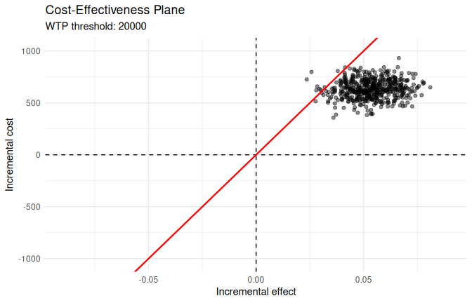
ceac_table <- computenmbceac(res_boot, wtp_range = seq(0, 50000, 5000))
head(ceac_table)
#> # basetable: 6 x 3
#>     WTP       ENMB Prob_CE
#> 1     0 -639.48888   0.000
#> 2  5000 -368.94762   0.000
#> 3 10000  -98.40636   0.224
#> 4 15000  172.13490   0.826
#> 5 20000  442.67616   0.982
#> 6 25000  713.21742   0.996
plotceac(ceac_table)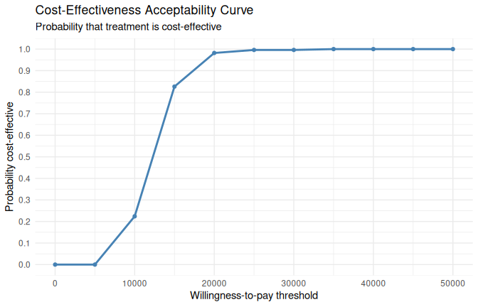
dsa_result <- dsaicer(cost + effect ~ group, data = trial,
                       param = "effect",
                       range = seq(0.74, 0.82, 0.02),
                       ref = "control",
                       metric = "INMB",
                       k = 20000)
dsa_result
#> # basetable: 5 x 2
#>   Parameter       INMB
#> 1      0.74 -320.20684
#> 2      0.76   79.79316
#> 3      0.78  479.79316
#> 4      0.80  879.79316
#> 5      0.82 1279.79316
plotdsa(dsa_result, metric = "INMB")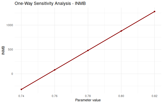
Trial costs and effects are often incomplete. micea()
runs the analysis in each completed data set and pools the incremental
cost, incremental effect, and INMB with Rubin’s rules (Barnard-Rubin
degrees of freedom). It accepts a mimar_imputation (from
mimar::impute()), a mids (from
mice::mice()), or a plain list of completed data frames.
The pooled CEAC table works with plotceac().
set.seed(1)
trial_mis <- trial
trial_mis$cost[sample(nrow(trial_mis), 50)] <- NA

imp <- mimar::impute(trial_mis, m = 5, seed = 1)
res_mi <- micea(cost + effect ~ group, data = imp, ref = "control",
                wtp_range = seq(0, 50000, 5000))
res_mi
#> Cost-effectiveness analysis pooled over 5 imputations
#> Reference: control; treatment: treatment; n = 400
#>
#> # basetable: 3 x 7
#>        Metric  Estimate StdError   Lower   Upper      df   FMI
#>    Delta Cost   661.826   92.720 479.342 844.311 291.696 0.061
#>  Delta Effect     0.054    0.011   0.033   0.075 398.000 0.000
#>          ICER 12231.525       NA      NA      NA      NA    NA
plotceac(res_mi$ceac)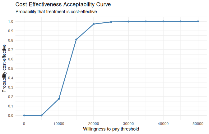
miboot() bootstraps first and imputes every bootstrap
sample with a user-supplied function (Brand et al. 2019). The result is
a booticer-compatible object, so
computenmbceac(), plotceplane(), and
plotceac() work unchanged.
impute_fun <- function(d) mimar::impute(d, m = 2)
res_miboot <- miboot(cost + effect ~ group, data = trial_mis, ref = "control",
                     imputefun = impute_fun, R = 100, seed = 1)
summary(res_miboot)
#> # basetable: 3 x 6
#>         Metric  Observed BootstrapMean StdError    Bias                    CI
#> 1   Delta Cost   686.372       659.151   98.374 -27.221    [462.925; 847.301]
#> 2 Delta Effect     0.054         0.057    0.010   0.003         [0.04; 0.081]
#> 3         ICER 12685.162            NA       NA      NA [7792.656; 16950.597]
plotceplane(res_miboot, k = 20000)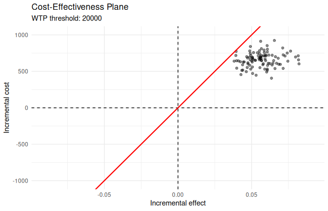
Both functions take an optional weights argument naming
a case-weight column (for example matching or inverse probability
weights computed within each completed data set).
CEACT also includes trial_cea, a 500-patient example
dataset with treatment, total cost, and QALY outcomes used in teaching
material for trial-based economic evaluation.
data("trial_cea")
real_res <- cea(cost + qaly ~ group, data = trial_cea, ref = "control")
summary(real_res)
#> Cost-Effectiveness Summary
#> Formula: cost + qaly ~ group
#> Reference group: control
#> Treatment group: treatment
#> Incremental cost: 25
#> Incremental effect: 0.042
#> ICER: 588.802
#>
#>              Outcome          Reference          Treatment Difference
#> delta_cost      Cost 3015 (SD 1582.802) 3040 (SD 1168.737)     25.000
#> delta_effect  Effect   0.573 (SD 0.217)   0.615 (SD 0.205)      0.042
#>                             CI p.value
#> delta_cost   [-219.54; 269.54]  0.8409
#> delta_effect [0.005; 0.08] 0.0251Unit tests are implemented with testthat.
Function documentation is generated with roxygen2.
A PDF vignette is available in vignettes/.
The package source builds and checks successfully with
R CMD check.