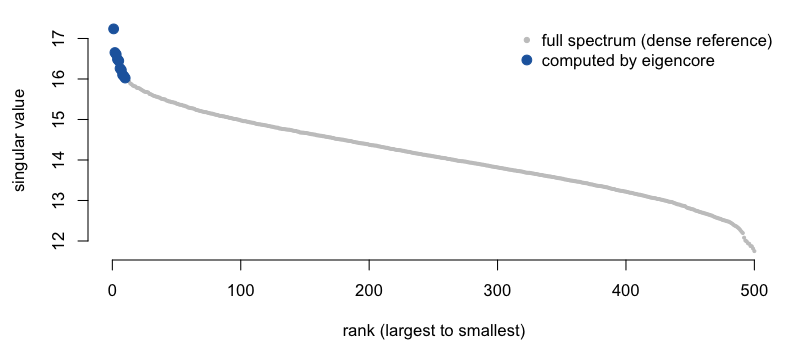
eigencore

eigencore computes the top-k singular triplets or eigenpairs of a large sparse or structured matrix in R — the computation behind PCA on big sparse data, spectral embeddings, LSA, and low-rank approximation.

eigencore focuses on two things:

1. Every result is checked. Each call returns residuals, a backward-error bound, orthogonality loss, and a single passed/failed flag. When a bound can only be estimated, the certificate says so instead of passing.
2. Centering and scaling without densifying. Explicitly centering a sparse matrix for PCA can require a dense copy. eigencore solves the centered (or scaled, or composed) problem as an operator, without forming that copy.

Supported structured problems run through fast native kernels. The Benchmarks section provides reproducible single-machine timings without treating them as cross-package rankings.

Installation

# install.packages("pak")
pak::pak("bbuchsbaum/eigencore")

Quick start

The top 10 singular triplets of a 100,000 × 500 sparse matrix — the core computation in sparse PCA and LSA:

library(eigencore)
library(Matrix)

set.seed(2)
A <- as(rsparsematrix(100000, 500, density = 0.002), "dgCMatrix")

fit <- svd_partial(A, rank = 10, target = largest())
fit
#> Partial SVD
#>   requested rank: 10
#>   converged rank: 10
#>   method: native certified Gram SVD special case
#>   target: largest
#>   max residual: 1.414065e-14
#>   max backward error: 4.474206e-17
#>   max orthogonality loss: 1.554312e-15
#>   norm bound: frobenius_exact
#>   scale estimated: FALSE
#>   certificate: passed

The printout names the kernel that ran, gives the worst residual, backward error, and orthogonality loss across the returned triplets, and shows the certificate passed with an exact norm bound. This problem uses the native certified Gram path; see Benchmarks for a reproducible timing on the development machine.

Certificates

An iterative solver can stop early, miss a cluster, or lose orthogonality and still return plausible-looking numbers. eigencore makes validation part of the returned result: it checks both singular relations (||A v - sigma u|| and ||A^T u - sigma v||) and exposes the evidence:

fit$certificate
#> eigencore certificate
#>   passed: TRUE
#>   tolerance: 1e-08
#>   type: residual_backward_error
#>   norm bound: frobenius_exact
#>   scale estimated: FALSE
#>   max residual: 1.414065e-14
#>   max backward error: 4.474206e-17
#>   max orthogonality loss: 1.554312e-15
#>   orthogonality tolerance: 1.490116e-08
#>   orthogonality required: TRUE

When the check cannot be made exact, the certificate says so. For a column-centered sparse matrix the only cheap norm bound is a stochastic estimate, so eigencore returns the singular values but sets passed = FALSE and tells you why:

cen <- svd_partial(center(A, columns = TRUE), rank = 5, target = largest())

cen$certificate$passed
#> [1] FALSE
cen$certificate$norm_bound_type
#> [1] "frobenius_hutchinson_estimate"
cen$certificate$notes
#> [1] "certificate scale uses a stochastic norm estimate; passed is withheld"

You decide whether an estimated bound is good enough for your analysis. The explicit flag lets downstream code distinguish an exact certificate from an estimate without inferring that distinction from solver convergence alone.

Center and scale without densifying

A dense centered copy of A would occupy 400 MB; the sparse original is a few MB. center() gives you the centered map as an operator, and the solver works through it directly:

A_centered <- center(A, columns = TRUE)        # a 100000 x 500 operator, not a matrix
svd_partial(A_centered, rank = 5, target = largest())$d
#> [1] 17.23701 16.65319 16.60961 16.48647 16.44760

Build operators with linear_operator(), combine them with compose(), crossprod_operator(), scale_cols(), center(), and friends. The planner picks the kernel from the structure; plan_solver() shows the choice before you commit to a long solve:

plan_solver(svd_problem(A_centered, target = largest()), rank = 5)$method
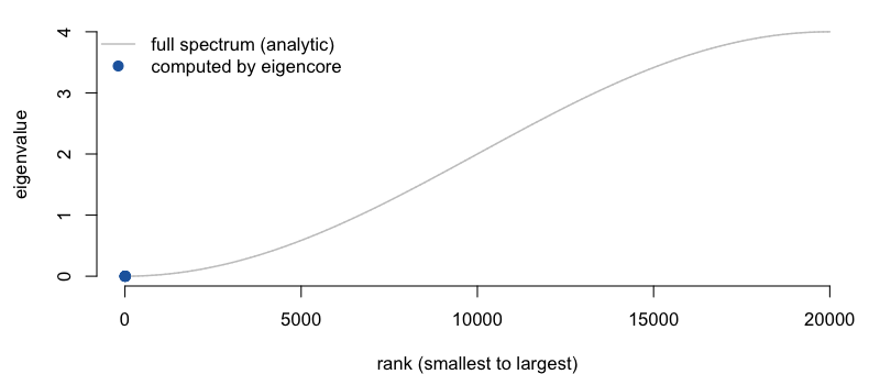
#> [1] "native matrix-free Golub-Kahan callback cycle + native Ritz extraction (callback boundary)"

Smallest eigenvalues of a symmetric operator

The same interface handles symmetric eigenproblems. Here is a sparse second-difference operator (a 1-D graph Laplacian) of size 20,000, asking for its smallest eigenvalues — the hard end of the spectrum for iterative solvers:

n <- 20000
L <- bandSparse(n, n, k = c(-1, 0, 1),
                diagonals = list(rep(-1, n - 1), rep(2, n), rep(-1, n - 1)))
L <- as(L, "dgCMatrix")

eig <- eig_partial(L, k = 8, target = smallest())
eig
#> Partial eigen decomposition
#>   requested: 8
#>   converged: 8
#>   method: native tridiagonal Hermitian shift-invert (factorized Lanczos)
#>   target: smallest
#>   restart: native_tridiagonal_shift_invert_lanczos
#>   locked: 0
#>   max residual: 9.026589e-10
#>   max backward error: 2.605774e-12
#>   max orthogonality loss: 4.884981e-15
#>   norm bound: frobenius_metadata+identity_exact
#>   scale estimated: FALSE
#>   certificate: passed

The planner selects a native tridiagonal shift-invert path and the resulting certificate passes. The exact spectrum is known in closed form, so the answer can also be checked directly:

Benchmarks

These are median wall-clock times for eigencore on one development machine. They include certificate computation and are intended as a reproducible performance smoke test, not a cross-package ranking or a performance guarantee. Reproduce them with Rscript inst/benchmarks/bench-readme.R.

_{Measured with R 4.5.1 on aarch64-apple-darwin20. Timings depend on the processor, BLAS/LAPACK, package versions, sparsity pattern, and workload; rerun the script before making performance decisions.}

The SVD rows use a bounded Gram kernel for tall or wide sparse problems whose small dimension is ≤ 512 (≤ 1024 for wide matrices). Other shapes may select different paths with different costs. fit$method always names the path that ran, making the relevant implementation boundary visible.

That path has fixed work associated with solving the smaller Gram problem and constructing a certified result. On the tiny examples used in documentation smoke tests, this overhead can dominate and RSpectra or irlba may finish sooner. As the long dimension grows while the smaller dimension remains within the planner boundary, the same path can cross over and become faster. This is a shape-specific effect, not a claim that eigencore becomes faster whenever a matrix gets larger; the benchmark vignette explains the comparison and its limits.

When to use what

Use eigencore for tall or wide sparse SVD (PCA-shaped problems), the smallest eigenvalues of banded or structured symmetric operators (certified, with automatic planner selection), centered or scaled or composed operators, dense generalized eigen/QZ/GSVD compatibility work through eig_full(), generalized_schur(), and generalized_svd(), and workflows where explicit certificate metadata is useful.

For workloads outside those structured paths, benchmark the candidate packages on your own matrices and hardware rather than assuming any implementation will be fastest. Side-by-side evaluation is straightforward because eigencore ships RSpectra-compatible wrappers with the same arguments:

res <- eigs_sym(L, k = 8, which = "SA")
res$values
#> [1] 2.467154e-08 9.868617e-08 2.220439e-07 3.947447e-07 6.167886e-07
#> [6] 8.881755e-07 1.208906e-06 1.578979e-06
res$certificate$passed
#> [1] TRUE

eigs(), eigs_sym(), and svds() accept the same which codes as RSpectra ("LM", "SM", "LA", "SA", "LR", "SR", "LI", "SI", "BE") and additionally return a certificate.

Learning more

• Get started with eigencore — the guided tour through partial eigenvalue and SVD workflows.
• PCA on sparse data without densifying — centered, scaled, and matrix-free sparse PCA.
• Reading certificates — residuals, backward errors, orthogonality, and withheld verdicts.
• Generalized eigenvalue problems — positive-definite metrics, dense pencils, QZ, and sparse partial solves.
• Benchmarks — reproducible comparisons, planner paths, and the limits of the timing evidence.

Status

eigencore 1.0.0 is headed for CRAN. The exported API is stable — it is frozen by a snapshot test, and breaking changes follow semantic versioning from here. Numerical behavior is covered by adversarial and reference tests, while solver results expose certificate and planner provenance on every call. Problem classes without a native kernel yet — general matrix-free SVD, interior eigenvalues at scale, nonsymmetric Krylov–Schur — are labeled reference in fit$method. The package vignettes describe the workflow map, benchmark evidence, and current boundaries.

License

MIT © Bradley Buchsbaum.